less pessimistic algorithm analysis
story of the amortized, 03 May 2019
why amortized analysis? the phenomenon of pessimistic analysis
Computer scientists should be familiar with Big-O, Big-Theta, and Big-Omega notation. They are notations explaining the upper and/or lower bound of asymptotic algorithm analysis. The word asymptotic is important since it emphasizes that the bound is relevant only on large enough and growing input size n, even as n is reaching infinity. In this context, we deliberately eliminate the need to calculate the actual running time. The case could be different if we know exactly that the input size will not be large enough and growing (in other words, stay relatively small at all times). Let’s take a story of two businessmen that we want to put our money into for investment. Business A has profit of 100 billion rupiahs, while business B has profit of 10 billion rupiahs (profit is analogous to actual running time). Some might directly choose to invest in business A, right? This decision could be right if both businesses are not expected to grow. However, this doesn’t even make sense in the case of investment, in which expected growth is what makes people invest at the first place. Further investigation on how the profit of both companies grow could change our decision, for example, profit of business A has been growing linearly while that of business B has been growing exponentially. So we can understand as the business grows (and the load scales), business B will eventually surpass business A in terms of profit, making business B more attractive target for investment. In the same way, the growth of runtime function determines which algorithm is more attractive to choose (as long as we expect large enough and growing input size).
However, there could be multiple answers to complexity problems. For example, runtime complexity for binary search algorithm (worst-case scenario) can have O(log2n), O(n) and O(n2). Those three, by definition, are correct though we all know that O(log2n) is the tightest one. For simple case like this, we can obviously detect that O(n) and O(n2) are too pessimistic. Yet, when we talk about a series of operations, this kind of too-pesimmistic approach is not very obvious. If we are unaware of it, we can produce an upper bound that is far higher than it really is, making our judgement inaccurate. There comes the help of amortized analysis. The purpose of amortized analysis is to produce more accurate assessment of algorithm complexity.
what is amortized analysis?
Amortized analysis is a method to gain deeper understanding towards the execution of a sequence of operations on a particular data structure. In this writing, we are going to discuss only aggregate analysis technique. The idea is that within a sequence of operations, one operation could have higher complexity/cost compared to other operations. And attributing this higher complexity to all operations within the sequence, while not necessarily wrong, could cause us to miss the tighter version and be content with the pessimistic result. Furthermore, the idea of aggregate analysis is simply to generate the total cost and divide the value by the number of operations within the sequence, resulting in average value. This average value will be called the amortized cost for each operation.
amortizedCost = totalCost / numberOfOperation
example
Let’s take this problem for example:
Given a linked list L with sorted integer values. Find the address of element with value equals to sqrt(i), which i starts from 1 to n. (do ceiling operation when sqrt() results in float).
Finding the address for certain value in linked list will require us to iterate through the elements. We can see that there are two operations here. One is doing the search for element with value of sqrt(i); second is to do that n times, from 1 to n. The first operation, in worst case, could result in O(n) (when i is a large number), while the second is also O(n). Both of them combined, therefore, will result in O(n2). This is not necessarily wrong; however, we can achieve tighter result by observing the execution.
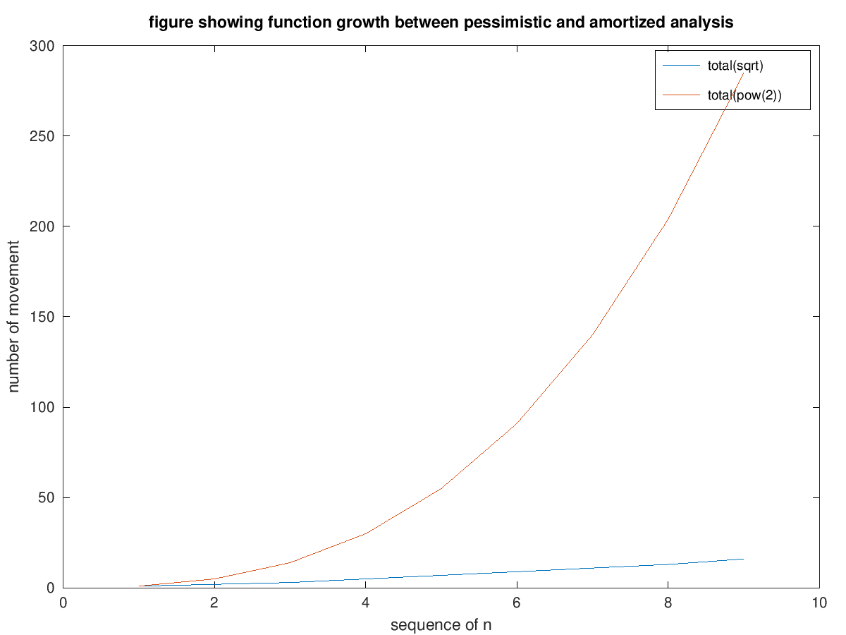
The table below shows the total movements required to find the address of the element: total(sqrt) and total(pow(2)). total denotes the accumulation from 1 to n.
| n | sqrt | total(sqrt) | pow(2) | total(pow(2)) |
|---|---|---|---|---|
| 1 | 1 | 1 | 1 | 1 |
| 2 | 1 | 2 | 4 | 5 |
| 3 | 1 | 3 | 9 | 14 |
| 4 | 2 | 5 | 16 | 30 |
| 5 | 2 | 7 | 25 | 55 |
| 6 | 2 | 9 | 36 | 91 |
| 7 | 2 | 11 | 49 | 140 |
| 8 | 2 | 13 | 64 | 204 |
| 9 | 3 | 16 | 81 | 285 |
The plot below (generated using Octave) helps us see that there is quite a gap between the real execution (blue) and our previous assessment (orange). There might be some room for improvement to come up with tighter upper bound.
I didn’t do the math computation to generate the new function as it’s out of the scope of this writing. However, by looking at this process, we can see that by doing observation to the real execution of a sequence of operations on a particular data structure, we might gain more understanding. This understanding might lead us to tighter algorithm complexity, resulting in better design decision.
Hope this is useful to you. Let me know if you have any to share in the comment section.